EDA PCB布线中的寻路智慧：深入探索Lee算法的可视化之旅

发布于 2025-05-28 18:43:55（微信公众号导出记录）。

本文来自公众号后台的“导出文章内容”功能。博客正文由导出长图进行本地 OCR 转写，并保留原始排版图用于逐段核对。

原文链接：查看原文

OCR 转写有效文字约 13902 字；代码、流程图和版式以文末原始排版图为准。

正文（本地 OCR 转写）

在现代电子产品设计的复杂世界中,EDA(电子设计自动化)工具扮演着至关重要的角 色。其中,PCB(印刷电路板)的设计是连接各个电子元器件、实现电路功能的物理载 体。一个常见的问题是:EDA工具是如何在密集的元器件之间,自动规划出那些婉蜓曲 折却又互不干扰的铜箔走线的呢?这青后其实隐着精妙的算法。本文将以PCB自动布 线中的一个基础且经典的寻路算法—-Lee算法(迷宫算法)为例,带你一起探索其工作 原理,并通过Python代码和可视化来直观感受其魅力。 从原理图到PCB:寻路的起点 在EDA工具中绘制PCB时,通常会先绘制电踏原理图(Schematic)。原理图定义了元器件之间的逻辑 连接关系,但并不关心它们的物理布局。当原理图转换为PCB布局时,EDA工具会根据元器件的物理封 装(Footprint)和原理至中的连接信息(通常通过网络表Netlist传递),在PCB板上放置元器 件,并在需要连报的引脚之间显示飞线(FLyLines/Ratsnest)。 这些飞线仅仅是逻辑连接的提示,它们相互交叉,杂乱无意。真正的挑战在于如何将这些飞线转换为实 际的、遵循各种设计规则(如最小问距、线宽,层限制等)的铜结走线。这就是自动布线器 (Autorouter)的用武之地,而寻路算法则是自动布线器的核心。 Lee算法(迷宫算法):如水波般探索 Lee算法,因其发明者C.Y。Lee而得名,也常被称为递宫算法或洪水填充算法、它是一种基于广度 优先接察(BFS)的网格寻路算法,以其完备性(只要路径存在就能找到)和最优性(在单位成本一 致时找到最短路径)而著称。 首先套一下效果 MP4: Drawing Path (Point 16/19)

1.核心思想

想象一下,在一个迷宫中,从起点滴人一滴水。水波会向所有可通行的方向均速扩敬。第一波到达的地 方距离起点为1,第二波到达的地方距惠为2,以此类推。当水波“滩没“终点时,我们就可以从终点沿 着水波退回的方向(即效字减小的方向)找到一条回到起点的最短路径。这就是Lee算法的直观理解。

2.算法步骤

:胃格化(Gridding):

• 可通过单元(Traversable Cells)

:标记为例如或一个特殊的“末访问“值(如-1)。 障碍物单元(Obstacles) :如元器件焊盘、已布好的其他走线、过孔、禁止布线区等,标记为例如1或一个特炼的 “险物”值(如-2)。

• 起点(Start Node)S

:路径的开始引脚。

• 线点(End Node)E

:路径的目标引脚。

• 将PCB的布线层(或多层空间)象成一个巨大的横盘或网格。每个小格子代表一个潜在的布

线单元。

• 标记网格

• 波前扩展(wave Expansion/ Propagation):

• 从队列头蕴取出一个单元格P(当前处理的单元格)。

■检查P是否为终点E。如果是,则路径已找到,可以结束扩展,进入回潮阶段。

• 对于P的所有有效邻居M(通常是上、下、左、右四个方向):

• 有效性判断

:邻居N必须在网格边界内、不能是障物、并且之前末被访问过(即其在 distance_grid 中的值仍为 - 1)。

• 标记与入队

:如果N 有效,美消其在 distancc_grid 中的距惠值设为 distancc_grid [P] +1 ,并记录P是N的父节点(用于后续路径回湖)。然后将N加入队列尾部。

• 初始化队列

:创建一个队列(通常便用collections。dcquc),并将起点5故人队列。在记票距 施的网格(我们称之为distance_grid)中,将起点5 的距离标记为0。

• 循环扩展

:只要队列不为空: 路径国测(Path Retracing):

• 从终点E开始。

■根据父节点记录,反向查找:找到E的父节点,再找到该父节点的父节点,依此类推。

• 将这条反向路径上的所有节点收集起果。

• 将收集到的节点顺序反转,即得到从起点5到终点E的最短路径。

• 如果成功找到终点E:

• 无路径:

• 如果队列变为空,但终点E仍未被访问到,则说明从5到E之间不存在可通行的路径。

3.可视化Lee算法的魅力曾

通过编程(例如使用Python和MatpLotLib库),我们可以将Lee算法的每一步执行过程都可视化出 采,这对于理解算法非常有帮助。 首先引入相关的头文件 inport nurpy as np 1nport matplotlib.pyplot as plt inport matplatlib.patheffects # For text stroke 1nport collections Inport time # For optional celays between steps # This line can be helpful in Jupyter Notebook for interactive plots, 8# but might require Installing loympl or enabling a specific backend. 9# For Colab, the defauIt Inline backend will show pTots after cell exe # or murltiple plots if plt.pause{) is used extensiveTy in a single ce] 11# amatplotlib notebook 12#atpotlIb Lpyapt 然后实现核心的lee_algorithm_visual_detailed

• -- I. Lee Algorithe Core Inplementation

def lec_algorithn_visual_detailed(grid, start, end, visualize_steps=Fa Lee Algorithn inplementation with step-by-step visualization of w8 cxpansion and path backtracking. Parameters: grid (np.array): 20 numpy array, for traversable, 1 for obstacle start (tuple): (row, col) coordinates of the start point. visualize_steps (bool): If True, visualizes after each expansion 5 fig_live (natplotlib.figure.Figure, optional): Figure object for 1. Returns: (path, distance_grid, wave_front_history) path (list): List of {row, col) coordinates for the path, or None. distance_grid (np.array): The final grid shoving distances fron th wave_front_history (list): List of grid states during wavefront ex) (if visualize_steps=False) . If True, th. night be inconplete as visualization is rows, cols = grid.shape Input validatfon 1f not (θ <= start[θ] < rows and e <= start[1] < cols and θ <= enc[θ] < rows and e <= end[1] < cols): print(fError: 5tart {start} or End {end} is out of grid bound return None, None, None if grid[start[θ], start[1]] == 1: print(fError: 5tart {start} is an an obstacle.") return None, grid, None if grid[end[0], end[1]] == 1: print(fError: End (end) is on an obstacle.") return None, grid, None fistance_grid = np.full((rous, cols], -1。 dtype=int) x -1l: unvisit; parent_grid = () Using a dictionary for porent tracking: ((r, c) wave_front_history - [] distance_grid[grid == 1] = -2 Mark obstacles queue = collections.deque() queue,append(start) distance_grid[start[0] . start[1]] = β if not visualize_steps: wave_front_history append (distance_grid.copy()) elif ax_live and fig_live: visualize_grid_live{ax_live, distance_grid, "Wave Step: Initia fig_live.canvas draw() plt.pause(1. 0) noves = [(-1, D), [1, @), (θ, -1), {θ, 1)] # Up, Down, Left, Righ path_found = Falsc step_count = 0 while queue: step_count += 1 curr_r, curr_c = queue-popleft(1 5 1. if (curr_r, curr_c) == end: path_found = Truc If visualize_steps and ax_live and fig_live: visualize_grid_live(ax_live, distance_grid, fWave 5te] fig_live,canvas.draw() plt. pause(0.5) break made_changc_in_this_cxpansion = Falsc for dr, dc in moves: next_r, next_c = curr_r + dr, curr_c + dc if e <= next_r < rous and e c= next_c < cos and distance_grid[next_r, next_c] = distance_grid[curr_r, parent_grid[(next_r, next_c)] = (curr_r, curr_c) queue.append((next_r, next_c)) made_change_in_this_expansion = True if visualizc_steps and ax_live and fig_live and made_changc_in. visualize_grid_live(ax_Llive, distance_grid, f"Wave Step [5 fig_live.canvas dras() plt-pause(&,1) Adjust pousc tinc to control aninotion sp el1f not visualize_steps and made_change_in_this_expansion: if not vave_front _history ur not np.array_equal (wave_fron wave_front_history.append(distancc_grid,copy()) aUON = 44ed 1eut↓ if path_found: [1 = q4edeu pua = Jn while curr != start: final_path.append(curr) If curr not In parent_grid: Safety check 8 1 print(f"Backtracking Error: Node fcurr} has no parent return None, distance_grid, wave_front_history curr = parent_grid[curr] final_path.append{start) final_path.reverse() 1f visualize_steps and ax_live and fig_live: visualize_grid_live(ax_live, distance_grid, "Final Path Fa fig_live,canvas drau() plt.pause (2.0) elif visualize_steps and ax_Live and fig_live: visualize_grid_live(ax_live, distance_grid, "No Path Found to f1g_live.canvas draw() plt.pause(2.0) return final_path, distance_grid, wave_front_history 接着实现可视化函数visualize_grid_live

2. Visuallzotfon Function (for Live updates or snapshots)

def visualize_grid_llve(ax, grid_data, titte, start_node=None, end_ned. visualizes the grid state live on the given Axes object. Clears the Axes and redraws everything. ax,clear() rows, cols = grld_data.shape Deterwine max distance for colonmap scaling valid_distances = grid_data[grid_data >= θ] 1f len(valid_distances) == 0: clsc: max_dist_int = 1nt(np.fLoor(np,max(valid_distances))) Colormap and Norwalization Selup -- Sasc colors: 0bstacle (-2), Unvisited (-1) f1nal_cmap_colors = [{0.2,0.2,0.21, 0bstacie - dark_grey Unvisited - white (1,1,1)1 Sasc boundorics for normalization final_bounds = [-2.5, -1.5, -0.5] Add colors and bounds for distances (o, 1, max_dfist_int) if max_dist_int >= θ: num_dist_colors = max_dist_1nt + 1 Use pll.gel cmap() to avoid MatplotlibDeprecationwarning dist_cnap = plt,get_cnap( *Blues', nun_dist_colors if nun_dist_ for 1 in range (num_dist_colors): if nun dist colors == 1: Only distance 9 (start point) color_val = θ,3 # A light bluc :8510 color val = i / (num dist colors - 1) α Nornalize i fc final_cnap_colors.append(dist_cnap(color_val)) final_bounds.append(1 + @,5] Upper bound for olstance I 3 2 custom cmap = ncolors .ListedColormap(final_cnap_colors) norm = mcolors,BoundaryNorm(final_bounds, custom_cmap.N) ax.Imshow(grid_data, cmap=custom_cmap, norn=norm, Interpolation=n Grid Lines and Text Annotations for r_idx in range(rows): # Thin grid Lines 4 1 ax-plot([c_idx - @.5, c_idx - @.5]. [r_idx - @.5, r_idx + 43 val = grid_data[r_idx, c_1dx] text_color = hlack # Default text color If val >= B: # If it’s a distance valve If val <= max_dist_int : # Check if val is a valid ind If color_idx_for_dist < len(final_cmap_colors): bg_cotor = final_cnap_colors[color_idx_for_dis' brightness = sum(bg_color[:3]) / 3.θ # Sinpie 1f brightness < B,45: # If background is dark text_color = 'white ax.text(c_idx, r_idx, Str(int(val)), va=′center, ha= obstacles are visually distinct by color, so x is opti ellf va[ == -2: ax.text(c_idx, r_idx, 'X', va='center', ha=*center Start/End, Current Wode, ond Path Markers pe = [matptotllb. patheffects.withstroke(Linevlath=2, foreground= b if start_node: ax.text(start_node[1], start_node[θ].“S', va=′center",ha='cc 1f end_node: ax.text(end_node[1]. end _node[θ]. E, va=′center', ha=*center r, c = current_processing_node rect = plt.Rectangle((c - B.5, r - @.5), 1, 1, linewidth=2, ed ax,add_patch(rect) 1f path_coords: If a path is provided, drav It path_c = [p[1] for p in path_coords] ax.plot(path_c, path_r, color=′orange , Linewidth=2.5, linesty Gptionally。 mark points on the path ax.scatter(path_c, path_r, color=*yellov', s=25, cdgecolor='bl.

• -- Final Axes Adjustiwents

ax.set_xticks(np.arange(cols)) Sel intermel lick positions ax,sct_yticks(np,arange(rows)) ax.set_yticklabels{[1) ax,tick_parans(axis=*both’, which=both’, length=B) Hidc tick mo ax.set_title(title, fontsize=10, welght= bold′) ax.set_aspect('equal', adjustable=bux) 然后实现仿真环境的迷宫构建与起点终点设定 Define the Grlo, Start, and End Nodes exanple_grid = np.array{ [ [, 8, 8, 0. 1, 0, 8, o, 0, e], [0, 1. 1. 0, 1. 0, 1, 1, 1, 0], [8, 8, 6, 0, 1, 0, 1, e], [1, 1, 6, 1, [0, 8. 0.0. 0. 0. 1. 0, 0. 0], [0, 1, 1, 1, 1, 0, 1, 1, 1, , [, 8, 8, 0. 1, 0, 8, o, 1, e], [0, 1. 1, 0, 0, 0, 1. 0, 1. 0], [θ, 1, 8. 0, 1, 0, 1, 3, 8, , [8, 8, 8, 1, 1, 0, 0, 0, 1, 0] start_node = (θ, 6) {row, col.) [row, col) cnd_node = (9, 9) # You can try different grids and start/end points here! # For t example: # sinplc_grid = np.orray( [ [0,0,0] , [0,8,0] W # star'[ node sinple = (θ,9] # cnd_nodc_sinplc = (2,2) 最后实现算法的快照回顾 Mode 2: Post-Execution Snapshot Visualization # This mode runs the algoriths first to collect atL Intermedlate state. # then displays key snapshots. This is generally more robust in Coiab/ print("\nExecuting Mode 2: Post-Execution Snapshot visualization...") # Run the algorithn vithout live visualization to collect history path_snapshot, final_dist_grid_snapshot, wave_history_snapshot = lee_a example_grid. copy() , start_node, end_node, visualize_steps=False Disable live steps to collect full vave_hf. # Smapshot I: InitiaT Grid fig_initial_snap, ax_initial_snap = plt,subplots(figsize=(7, 7)) Initial_display_grld_snap = np-full(example_grid.shape, -1, dtype=1nt) 14 if start_node: initial_display_grid_snap[start_node[θ] , start_node[1]] sdeus, deusptu6Ae1dstp1etatut deus1etatutxe)aAtiptu6aztlen5A fig_initial_snap-tight_layout() plt show() # Snapshots 2: Wave Expansion (selected steps) if wave_histary_snapshot: num_wave_steps_total = len(wave_history_snapshot) Select a fev representative snapshots to disptay if mum_wave_steps_total > 5: Shov first, a few in middlc, and last Indices_to_show = np.unique(np.Linspace(0, num_wave_steps_tota if nun_mave_steps_total -1 mot in indices_to_show: # ensure Ia. indiccs_to_show.append(num_wavc_stcps_total -1) Indices_to_show = sorted( List(set(indices_to_show))) else: indices_to_show = rangc(nun_wave_steps_total) for 1, step_idx 1n enumerate(indices_to_show): [xp da1s] 1oysdeus fuo1stq axen = 1ousdeus pJ6 #Aex fig_wave_snop, ax_wave_snap = plt, subplots(figsize=(7,7)) title_str = f"snapshot: 2.[1+l} Wave Expansion [Record (step_1 Check if largel is reached in this specific snapshot is_targct_rcached_in_this_snap = (path_snapshot and wavc_grid_ More accurately. check If this Is the first snapshot where if is_target_reached_in_this_snap: if stcp_idx == @ or (step_idx > 0 and vave_history_snapsho title_str += '- Target Reached in this step!" 4 1 elif wave_history_snapshot[step_idx-1][end_node[@]. end_no Target Previously Rcached title_str 4= *. visualize_grid_live(ax_wave_snap, wave_grid_snapshot, title_st fig wave snap.tight_Layout(1 plt,show() Snapshot 3: Flnal Path or No Patih If path snapshot: fig_final_snap, ax_final_snap = plt,subplots(figsize={7, 7)) v1sualize_grid_live(ax_final_snap, final_dist_grid_snapshot, Snap fig_final_snap.tight_Layout() plt show() print(f"\nPath found (snapshot model: ({path_snapshot]") print(f"Path length: {len(path_snapshat) -1} steps") elif final_dist_grid_snapshot is not None: # Even if no path, shov the shov the f1g_no_path_snap, ax_no_path_snap = plt.subplots (figs1ze=(7,7)) visualize_grid_live{ax_no_path_snap, fina1_dist_grid_snapshot, fig_no_path_snap. tight_layout() plt show() print("nNo path found (snapshot mode).) "ynError during snapshot mode exe e1dstp o1 ptu6 ou Snapshot: 1. Initial Grid

Snapshot: 2.1 Wave Expansion (Record 1/40)

Snapshot: 2.2 Wave Expansion (Record 10/40)

hapshot: 2.3 Wave Expansion (Record 20/40)

Snapshot: 2.4 Wave Expansion (Record 30/40)

shot: 2.5 Wave Expansion (Record 40/40) - Target Previously Reached Snap

Snapshot:3. Final Path Found

4.算法特性分析

优点:

• 完备性

:只要物理上存在路径。Lee算法一定能找到。

• 最优性

:在所有“步”的成本都相同的情况下(例如,在网格中移动一格的成本为1),Lee算法保证 找到的是几何上最短的路径(如经过最少单元格的路径)。

• 概念简单

:相对于一些更复杂的启发式算法,Lee算法的逐辑直观易懂。 缺点:

• 内存消耗

:需要一个与布线区域同样大小的数组来存储距离信息,对于大规机、高精度的PCB,内存开 销巨大。 计算时间 :当起点和终点距离很远,或速宫非常复杂时,波前需要扩展到几乎所有可达区域,计算耗 时较长。

• 路径形态

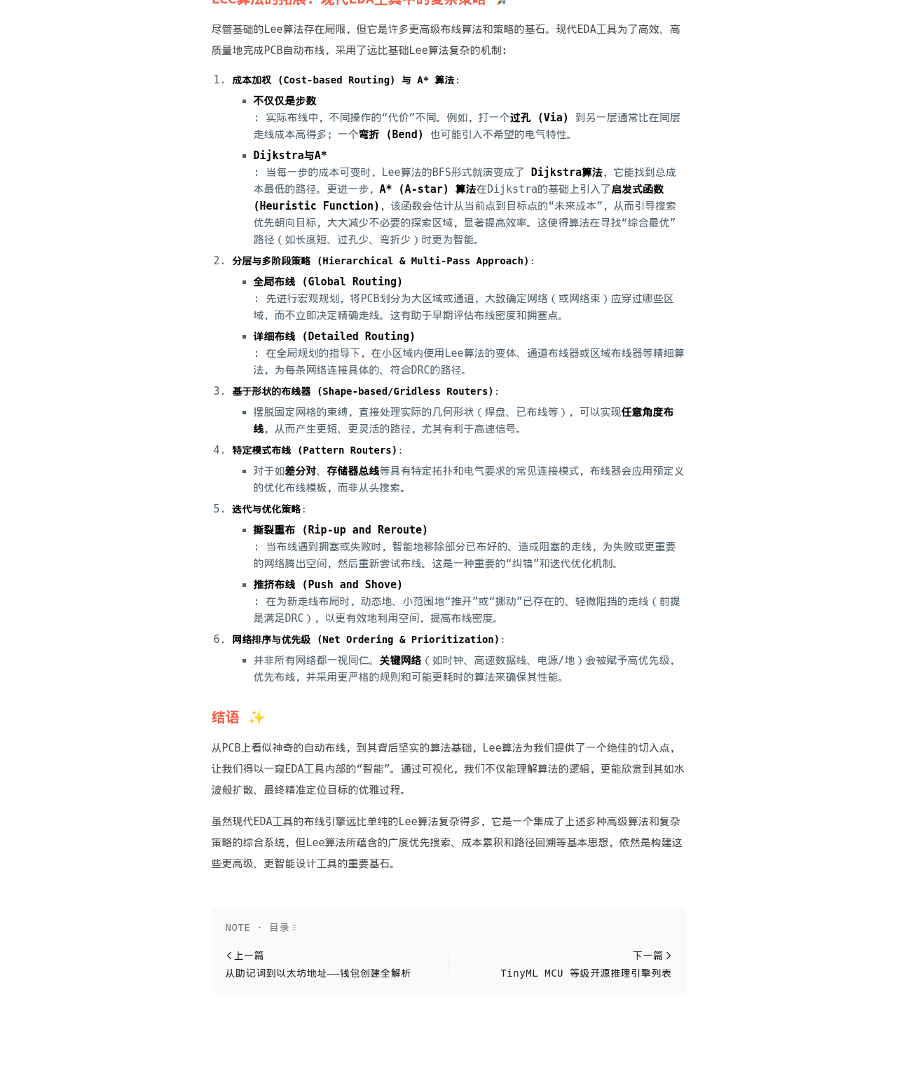
:倾向于产生曼哈顿式的直角转弯路径,可能不是电气性能最优的(例如,45度转角通常更 好)。 Lee算法的拓展:现代EDA工具中的复杂策略1 尽管基础的Lee算法存在局限,但它是许多更高级布线算法和黄略的基石。现代EDA工具为了高效、高 质量地完成PCB自动布线,采用了远比基础Lee算法复杂的机制:

1.成本加权(Cost-based Routing)与A*算法:

:不仅仅是步数 :实际布线中,不同操作的“代价“不同。例如,打一个过孔(Via)到另一层通常比在同层 是线成本高得多;一个弯折(Bend)也可能引人不希望的电气特性。 = Dijkstra与A* :当每一步的成本可变时,Lee算法的BFS形式就演变成了Dijkstra算法,它能找到总成 本最低的路径。更进一步,A*(A-star)算法在D1jkstra的基础上引入了启发式函数 (HeuristicFunction),该函数会估计从当前点到目标点的“未来成本”,从而引导提索 优先朝向目标,大大减少不必要的探索区域,显若提高效率。这使得算法在寻找“综合最优” 路径(如长度短、过孔少、高折少)时更为智能。

2.分展与多阶段繁路(Hierarchical & Hulti-Pass Approach):

• 全局布线(GLobal Routing)

:先进行宏观规划,将PCB划分为大区域或通道,大致确定网络(或网络束)应穿过哪些区 域,而不立即决定精确定线。这有助于早期评估布线密座和拥塞点。 :详细布线(Detailed Routing) :在全局规划的招导下,在小区域内便用Lee算法的变体、通道布线器或区域布线器等精细算 法,为每条网络连接具体的、符合DRC的路径。

3.基于形状的布线器(Shape-based/Gridless Routers):

• 摆脱固定网格的束绒,直接处理实际的几何形状(焊盘、已布线等),可以实理任意角度布

线。从而产生更短,更灵活的路径,尤其有利于高速信号。

4.特定横式布线(Pattern Routers}:

对于如差分对、存储器总线等具有特定拓扑和电气要求的常见连接模式,布线器会应用预定义 的优化布线模板,而事从头提蒙。

5.选代与优化策略:

• 撕裂重布(Rip-up and Reroute)

:当布线遇到拥霆或失败时,智能地移除部分已布好的、遗成阻塞的走线,为失败或更重要 的网络腾出空间,然后重新尝试布线。这是一种重要的“纠错”和选代优化机制。

• 推挤布线(PushandShove)

:在为新走线布局时,动态地、小范围地“推开"或“挪动"已存在的、轻微阻挡的走线(前提 是满足DRC),以更有效地利用空间,提高布线密度。

6.网络排序与优先级(NetOrdering&Prioritization):

■并非所有网络都一视同仁。关键网络(如时钟、高速数据线、电源/地)会被赋予高优先级, 优先布线,并采用更严格的规则和可能更耗时的算法来确保其性能。 结语 从PCB上看似神奇的自动布线,到其背后坚实的算法基础,Lee算法为我们提供了一个绝佳的切入点, 让我们得以一窥EDA工具内部的“智能”。通过可视化,我们不仅能理解算法的逻辑,更能欣赏到其如水 波般扩散、最终精准定位目标的优雅过程。 虽然现代EDA工具的布线引擎远比单纯的Lee算法复杂得多,它是一个集成了上述多种高级算法和复杂 策略的综合系统,但Lee算法所蕴含的广度优先搜索、成本累积和路径回溯等基本思想,依然是构建这 些更高级、更智能设计工具的重要基石。

NOTE·目录三 <上一篇 下一篇> 从助记词到以太坊地址--钱包创建全解析 TinyMLMCU等级开源推理引擎列表

原始排版图

原始导出图超过单张 WebP 的尺寸上限，以下图片按从上到下的顺序连续保存。